Mathieu GT

Today we will talk about statistics applied to biodiversity

During this course, we talk a lot about indices and measures of biodiversity, and we mentioned some statistical concept and tests that can be applied to the study of biological diversity. Today, I will show you some of them, and how they can be used. So, let’s start from some basic concepts. What are mean, median, and mode in statistics? When we describe quantitative data is often necessary to perform some fundamental analysis in statistics, where to measure out a set, we need to analyze their central tendency and their distribution. The arithmetic mean is a type of mean that is most commonly used for the analysis of the central tendency and what to which in determining is usually referent in statistic.

 It is used as a summary of the data site or the measurable phenomenon, for example, the i of the trees. This means it’s just calculating by adding the different values available xi, which are divided by their total number n. The formula is simply the sum from 1 to n of xi divided by n. In the case where it’s necessary to calculate the mean from a group of data in frequency table called f.

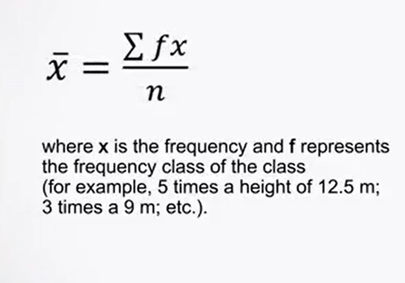
This may be calculated from the formula, the sum of fx divided by n where x is the frequency and therefore represents the frequency class, for example, 5 times of an i of 12.5, not 3 times of an i of 9, etc.

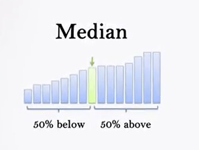
Median is the value assumed by statistical units that are located in the middle of the distribution. The median, in fact, is the central value of a series. So, it can be calculated by distributing the data in ascending order and identifying the value above and below which there is an equal number of data

When data are in equal number, the median is constituted by the average of the two values that formed a central pair.

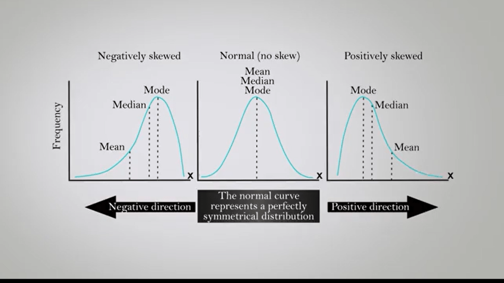
That mode, instead, is the maximum frequency value, and is often represented with the v0 sign mode. In other words, it is the value that appears most frequently. A distribution is unimodal if it emits only one mode of value. It is bimodal if it emits two. That is, that if there are two values, they appear both with a maximum frequency in the distribution date. If the graphs are useful to the term in the model class, identifying the maximum high interval, which is the maximum point of the curve. The class with the highest mean density, which corresponds to the high of the histogram is modal.

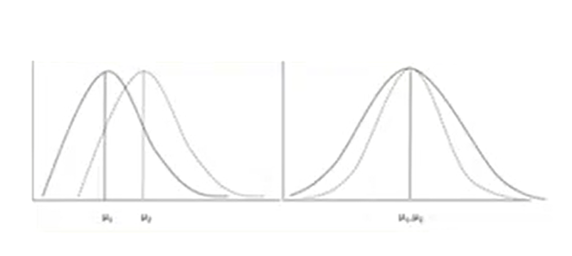
In the particular case of the normal distribution, also called Gaussian distribution, the mode coincides with the mean and the median. The normal distribution quote is used for me to analyze the distribution of data, and we can use the probability density function It represents the density of a continuous random variable and describes the relative probability that the variable falls within a range of values. The normal distribution is considered the ultimate example of continuous probability distribution because of its role in the central limit theorem. The normal or Gaussian distribution isa continuous probability distribution which is often used as the first approximation to describe random variables with actual value, that tend to distribute around a single mean value. The graph, or the probability density function associated to a normal distribution is a metric and has a bell shape known as normal curve or bell curve.

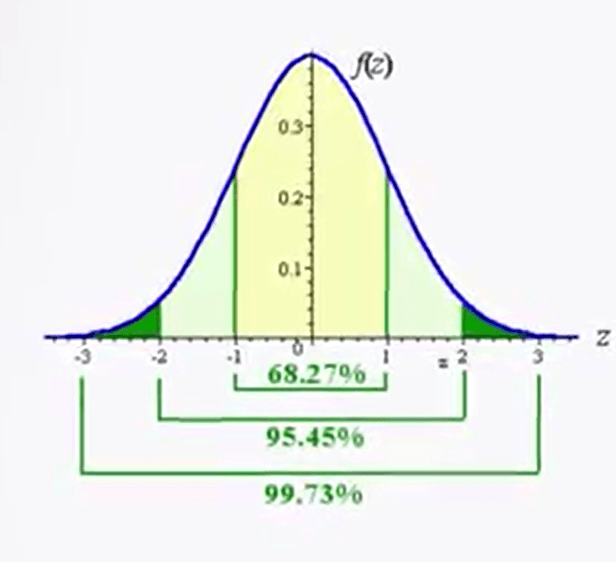
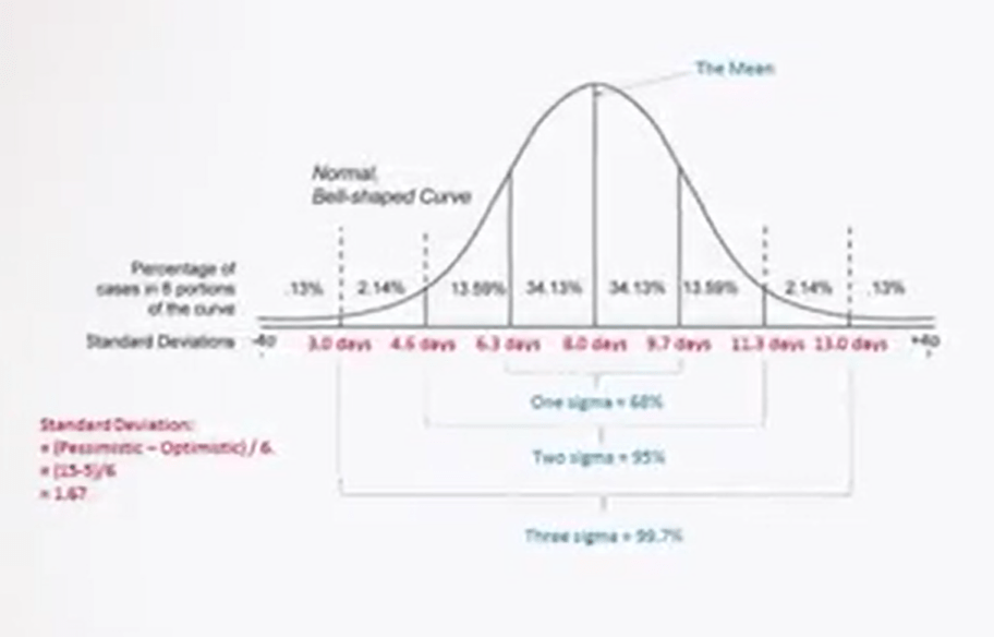
The normal distribution depends on two parameters, the mean and the variance, and is indicated in the following way. The normal curve is symmetrical, and its axis of symmetry passes at exactly through the intermediate point of the adjacent and corresponds to the mean, the median, and the mode of the data. On each side of the curve, there is an inflection point. The distance of the point of inflection from the central axis, the mean, can be used as you need of standard deviation or distance. As can be seen by observing the figure in the picture, each segments represent a unit of standard deviation. And if we consider that the total area below the curve represent 100% of the data, they are detected by each segment of +- 1 as d or standard deviation correspond respectively to 68%, 95.44%, 99.74%, etc. Since 95% of all observation will be within the range bounded by 1.96 +- sd, and 99% of all observation will be within the range bounded by 2.58 +- sd, the probability that any observation extracted a random from a sample falls outside the two intervals. They’re limited by this range, is respectively p 0.05, or p 0.01.

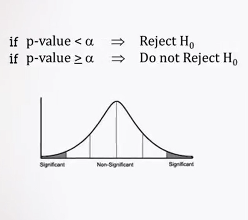
These values are the basis for the validation of statistical significance, and they are what is reported usually in any scientific paper. It is defined the probability distribution of zed. It is usual, in fact, to determine the statistical significance of a comparison test between the means or the medians of two samples, defining a null hypothesis, H0. This is simple, that the samples belong to the same population, and that their differences are due to shunts, rather than a systematic overall sampling. While the hypothesis H1 represents a possibility, then the samples belong to a specific population.

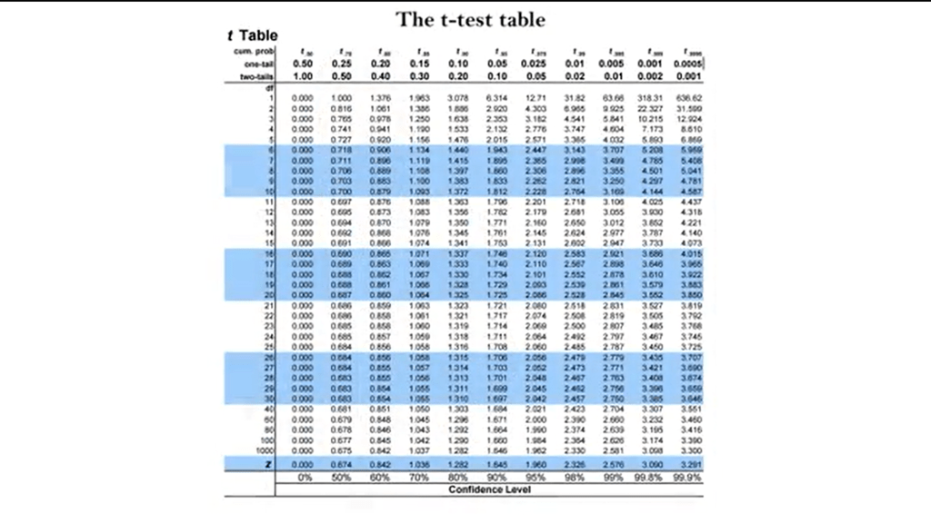
If other variables, such as, for example, the differences between male and female individuals are introduced by providing two direction for test the new hypothesis, the test is defined in two-tails test. In case you want one just to see whether the new hypothesis is confirmed or if it directed toward a single verification, H1, it is called one-tail test. Each statistical tests the levelof significance is measured by p 0.05 in correspondence to the value zed 1.65. That is less accurate thana two-tailed test for which zed is 1.96 or a level that is p 0.01 or p 0.001, which represent 5%, 1% and 0.1% of the values under the normal curve.

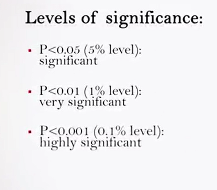
So there are three levels of significance, significant, very significant, and highly significant.

In statistical test, a value higher than zed 1.65 in one tail or 1.96 in two tails is statistically significant and does allow rejecting the new hypothesis that established the, for example, that the two samples come from the same population. We can say that the difference of the mean values between the samples is statistically significant, p less 0.05 or very significant where is p is less than 0.01, or highly significant where p is less than 0.001. And therefore, it is possible to reject the new hypothesis and to accept the alternative hypothesis H1.

Since the one-tail test is less stringent, unless there are specific reason, it is recommended to always use two-tails test, remembering that a significance in the two-tails test automatically means a significance in one-tail tests. So that’s all for the first part of statistics applied to the study of biological diversity, and see you at the second part.

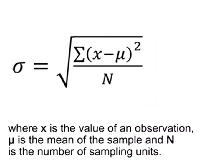
the standard deviation, is a measure of variation around the mean of the sample, and it can be calculated in the following way. In this formula, you see that xis the value of an observation, mu is the mean of the sample, and N is the numbers of sampling units. The numerator of the radical is defined of deviance. When the data are grouped by frequency values, it is needed to multiply the frequency f to the numerator of the radical. The variance, however, is simply the square value of the standard deviation, as indicated by a sigma square or s square.

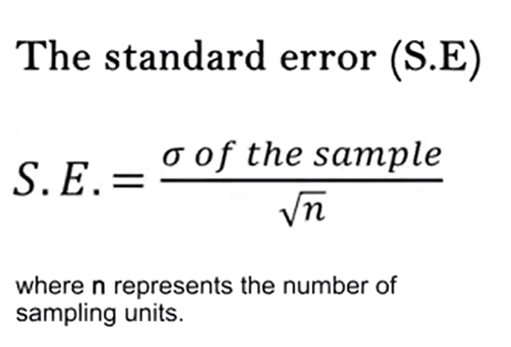
The standard error from the mean indicate show much the mean of the sample is close to the population mean. The standard error is simply the sigma or the s o the sample divided by the square root of n, where n represents the number of sampling units.

It makes no sense to report a mean without providing an indication of the associated standard deviation, or standard error. So, it is important, therefore, to always write that the sample as a mean of x plus or minus an sd, or plus or minus a standard error. When the variance of a sample is considerably higher than the mean, we have a case of aggregate data. In nature, aggregate random or uniform distribution of data can be observed. Because vary measured varies in ecology and in particular in the study of the biodiversity are asymmetrical as in normal the distribution, it is necessary to process the data. With this operation we obtain a compression of the asymmetric days. In other words, we squeeze the distribution to get a normalization of values. Distribution in this way acquires the same properties of a normal distribution and the same narrow limits can be used for the statistical analysis, as described in the previous lecture, to 95% or to 99%.

So, the probability of 0.05 or 001. The most useful transformation, when there are aggregates valued with greater variance from the mean, and no uniform, or symmetric distribution, is the logarithm transformation. That is to recalculate all the sample values transforming them with the log ten or the natural logarithm. If the variance is approximately equal to the mean, the distribution is defined random or Pearsonian. In these cases, the transformation with the square root is the most adequate. Sometimes it can be useful to adopt the arcsine transformation when the data are expressed as relative or percentage frequencies. In this way, the values will be scattered and included in a range between zero and one. Some statistical tests, nonparametric required to use of ranks. These latter are nothing more than an alternative system for classifying data. To assign ranks, all the data are listed in ascending order, ascending order depending on the test requirements. And to each one an integral value from 1 to N, the total number of sample units is assigned.

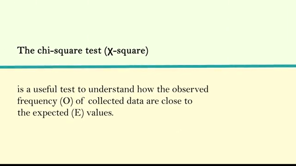
 The chi-square test is a useful test to understand how the observed frequency of collected data are close to the expected values. This test is frequently used although itis simple in the formulation it is not easy in calculation.

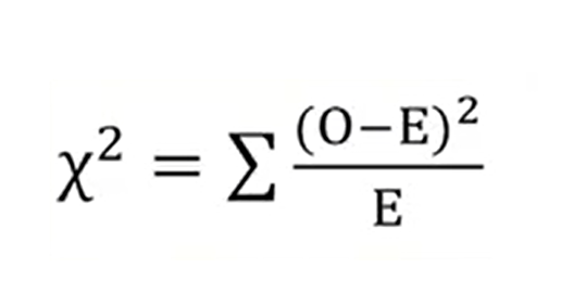
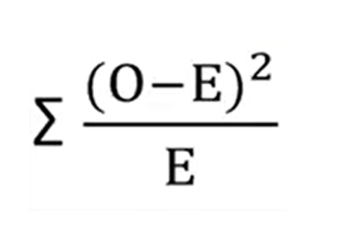
This formula is the following in just the sum of the square of several minus expected values divided by the expected values. This test is a kind of confrontation of the new hypothesis H zero. Because it provides that even in the for2, all the expected frequencies would be equal if the observant values were the result of of something else. For the practice of the calculation of the expected frequencies, just divide the sample of all frequencies detected in the samples, for example, the number of spiders caught in traps a, b and c, to the total number of samples in this example, r3. Then the observer frequencies correspond exactly to the number of units in the example. In this case, number of spiders in A,B and C traps.

We proceed to calculate the square value of the seven minus expected divided by expected values foreach samples A, B, and C and then the shareable that is updated from the sample, she’s then calculated. Then we need to calculate the doubles of freedom. That is the number of categories of the samples, minus one. Now our example is 3- 1, so 2. Then we take the value obtained from the calculation of the chi-square and the degree of freedom and we look at the test table that’s presented in any statistical book or online.

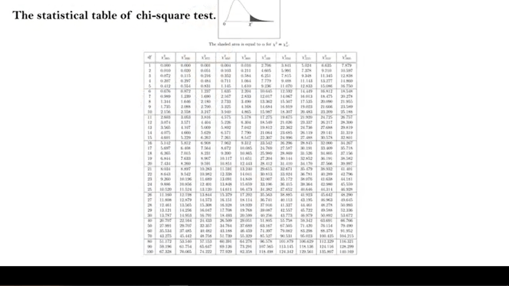
In the first column of this table there are degree of freedom and we can select and find those corresponding values to our. In our example, there are two.

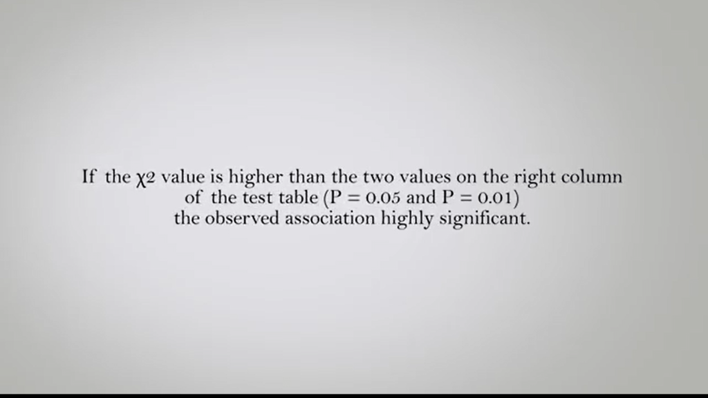
If the chi square value, we obtain is higher then the two values on the right column of the test table. Which contains the three short values for the probability 0.05 or 0.01. It can be concluded that the observed association between the frequencies and the related samples is highly significant. In the example, the trap with the higher number of spiders captured is significantly more effective in capturing these animals, if compared to the other two tested.

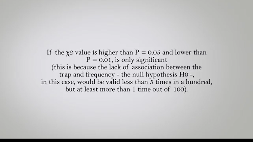
If the chi squared value were onlyhigher than the table value of P 0.05, and lower than P 0.01 this isassociation between frequency and sample would be only significant. This is because of the lack ofassociation between the trap and frequency that is the null hypothesisH0 In this case, would be valued less than five times in hundred but atleast more than one time out of hundred.

It is important to rememberthat this test is effective only if the expected frequencyexceeds the value of five. You can bypass this issue by aggregatingtwo or more categories of samples.

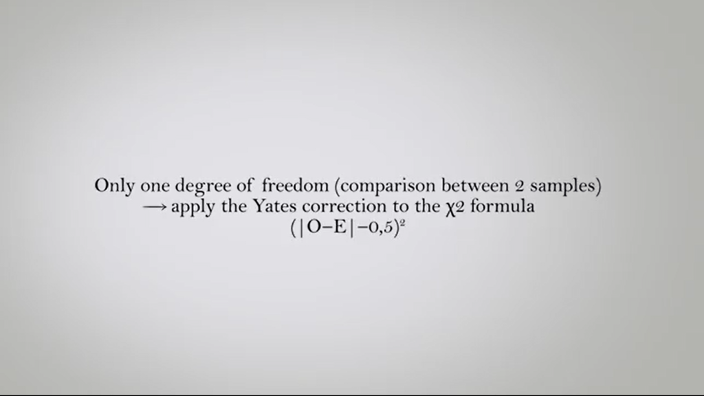
When there is only one degree of freedom, comparison between two samples, for instance, it is necessary toapply to the chi-squared formula the Yates correction for continuity, which simply consists in subtracting 0.5 to the numerator of the formula.

When we are conducting statisticalcomparisons between two samples, beside to be interested in the association between the observed frequencies and the effectiveness of the sample itself. So trap, sampling techniques, and so on, as explained in the previous lecture, one of the questions to answer inorder to demonstrate the validity of our hypothesis is if the sample size is significantly different, from a statistical point of view,of course. For example, if the biodiversity ofa contaminated site is statistically different from that of a non-contaminated site, it can be, in fact, that samples with a similar mean or median, can have completely different variances.

In general, the comparison tests between the samples are divided into non-parametric tests and parametric tests, depending on if they are comparing the means or the variances using actual values, orthe medians using ranks respectively. I would describe you some simple parametric test. This test assumes the observation are at scale of internal ratio, so they are continuous, otherwise the data should be transforming with the logging being transformation. And that they are deprived from the population normally distributed. If the distribution is not symmetrical, or you are not sure about that, you must use a nonparametric test. Generally biometric measurements, weight, height, length can be considered normal distributed when applied to homogenous categories, or male or female or adults or young people, for instance, while the are likely to be symmetrical. Before proceeding to the comparison of samples with a parametric test, you must make sure that the two samples are actually or probably extracted from the two different populations. Because although they can have similar means, at least the variances have to be different. Otherwise, you would have immediately confirmed the new hypothesis.

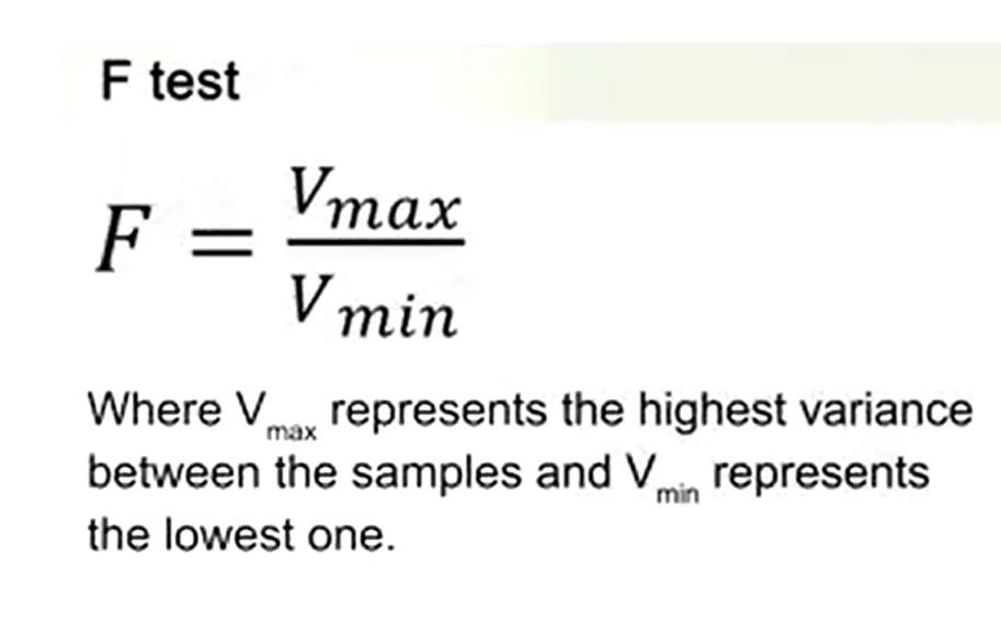
To check this issue, proceed to conduct a preliminary test that’s called F-test which evaluates the deviation of the ratio of two variances. So the F-test is just calculating that’s the maximum variance divided the minimum variance.

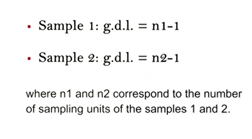
After calculating the variancesof the two samples, as described in the previous lectures, derive the degrees of freedom. So for the sample one is just degree of freedom minus one, and sample two the same, where n1 and n2 correspond to the number of sampling units of the samples 1 and 2.

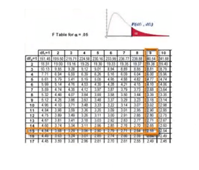
Subsequently, check into the distribution of the F-probability table the value at the intersection of the two degree of freedoms. If the obtained value of F is lower than that in the table, it is not possible to reject the new hypothesis immediately.

So, the variances are similar, because probably the two samples come from the same population, that is no statistically significant differences. We need to conclude that at this level ofanalysis, the two variances are similar and to accurately reject the null hypothesis and so confirm the statistical significance, we must proceed to perform a parametric test. Even the calculated value of F is higher than the critical value in the table for the respective degrees of freedom, is not necessary to proceed further, and it can be concluded that the null hypothesis is reject because the samples are significantly different. They do not derive from the same population. So only in the first case, the following test should be carried out.

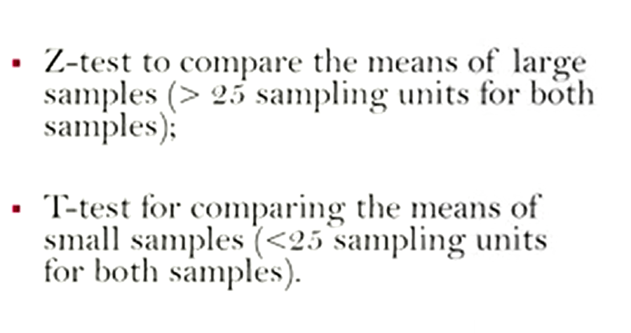
We can conduct the Z-test to compare the means of large samples. It means more than 25 sampling units for both samples, or we can carry the T-test for comparing the means of small samples. It means less than 25 sampling units for both samples.

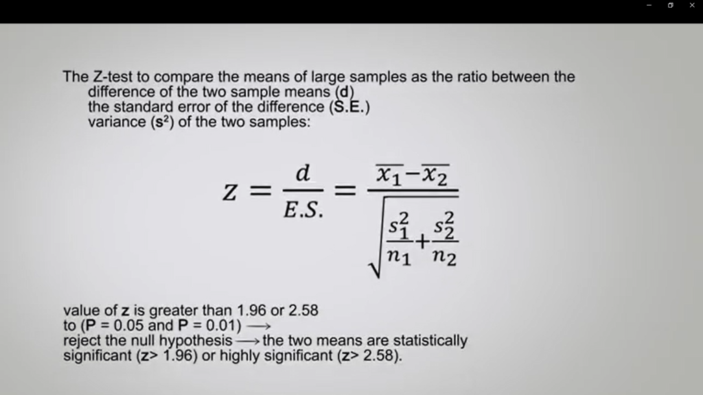
Z-test to compare the means of large samples as the ratio between the difference of the two samples means, and the standard error of the difference estimated from the variance of two samples can be calculated with the following formula.

If the calculated value of that is greater than 1.96 or 2.58, which is the normal distribution corresponding to P 0.05 or P 0.01, you can reject the null hypothesis and confirm that the two means are statistically significant or highly significant respectively.

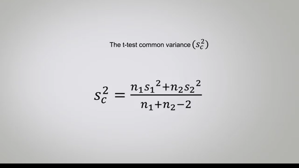
The T-test instead is useful to compare the means of small samples, and that’s used at the variance of the two samples being small, may be similar, and the sample units of both can be added up. So, this test introduces in the formula, the common variance,

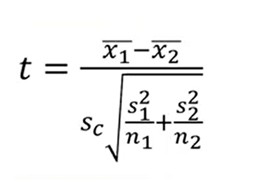
therefore, the formula becomes using the square root of the common variance, the following.

Checking in the probability table of these distribution, if the calculated value is larger than that in the table for the related degrees of freedom of a two-table test, you can reject the new hypothesis, and it can be concluded that the difference between the two means is significant.

T is more than the value in the table for P 0.05, or highly significant, T is greater than the value in the table to P 0.01.

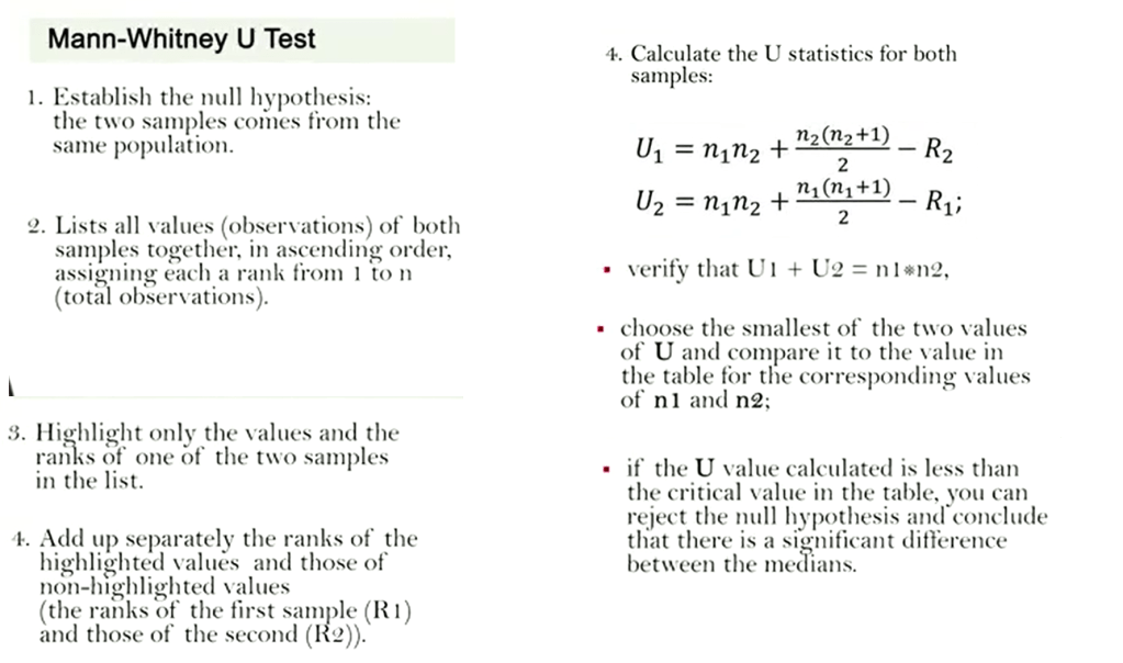
This time we see how to use non-parametric tests and comparison between medians. Non-parametric or independent from the distribution tests are those tests that did not require special conditions to be applied, do not need normal distributional data, should not be scaled or be in relationship. Anyway, when distribution is similar to the normal distribution, parametric meters are more efficient estimators. These tests are particularly suited to compare various more samples. One of the most used non-parametric tests is Mann-Whitney U test. This test allows the analysis of ordinal data to compare the medians of two independent samples. To calculate the test, you need to proceed as follows. First, establish the null hypothesis, that the two samples come from the same population. Then list all values your observation of both samples together, in ascending order assigning each a rank from one to n,that is the total of the observation. Then highlight only the values and the ranks of the one of the two samples in the list. Then add up separately the ranks of the values highlighted and those of non highlighted values. So, the ranks of the first sample R1 and those of the second sample R2.

And then you need to calculate the U statistics for both samples that is shown with the formula in this picture.

So, you need then to verify that U1 plus U2 is equal to n1 multiplied by n2. Then you need to choose the smallest of the two values of U and compare it to the value in the table for the corresponding values of n1 and n2. If the U value calculated is less than the critical value in the table, you can reject the null hypothesis and conclude that there is a significant difference between the medians.

Please pay attention to the fact that this is the only test for paired data that to reject the null hypothesis must have good calculated value lower than the critical one in table and not higher. When there are samples with more than 20 sample units, it is necessary to covert the smallest value of that in U. Let us bring back the statistical task of the normal curve.

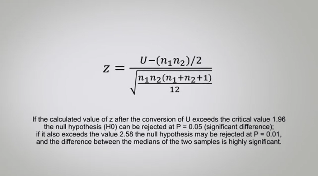
To do this, we add up the following formula. If the calculated value of zed after the conversion of U exceed the critical value of 1.96, the null hypothesis H0 Can be rejected at P=0.05 that there is a significant difference. If it also exceed the value at 2.58 the null hypothesis may be rejected at P=0.01, and the difference between the medians of the two samples is highly significant.

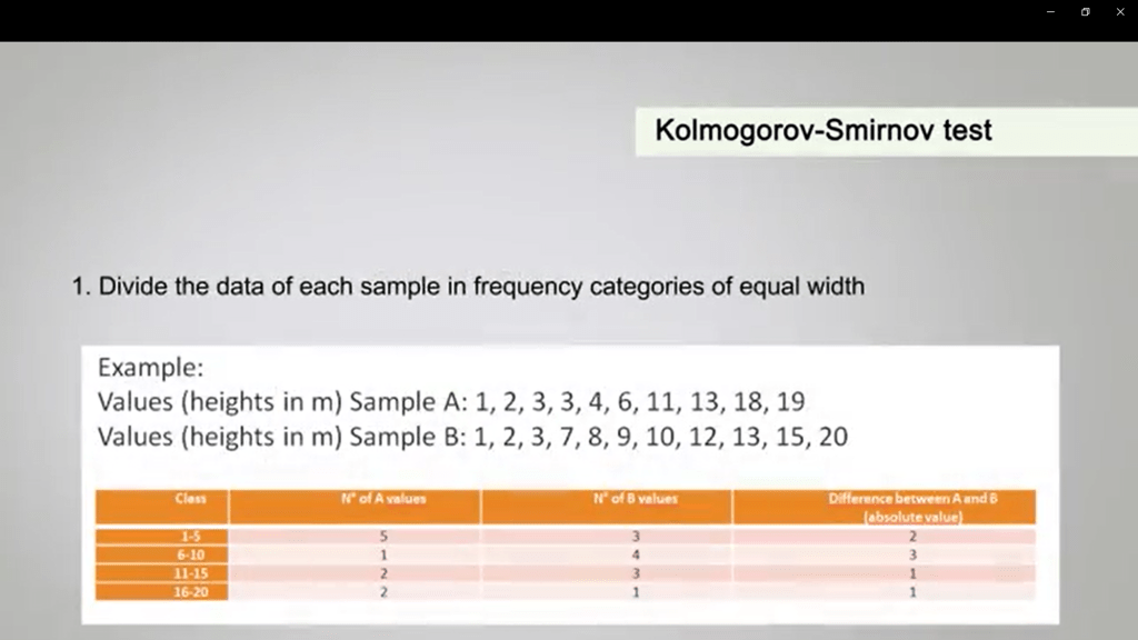
Another useful non-parametric test when you want to compare two samples is the Kolmogorov-Smirnov test. The Kolmogorov-Smirnov test allows you the comparison of quantitative data, and to calculate it you need to proceed as follows. First of all, you divide the data of each sample infrequency categories of equal width. In the example that Is how you in this table, you can divide the heights in five meter, in five. So, it means that one category is 1,5, the second one is 6, 10, the third one is 11, 15 and the fourth one is 16, 20.

For each class you attribute the community frequencies of the first and second sample. So, you add up how many values of each sample belong to each class. So, in the example, you will see that for class 1, 5 of the sample, A, there are five values. In the sample B, there are three. So, you look at the table andyou understand how distribute this value.

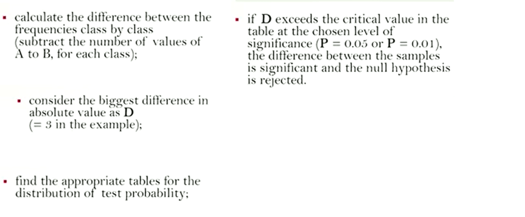
Then you need to calculate the difference between the frequencies class by class just to track the number ofvalues A to B for each class.

Then consider the biggest difference in absolute value as D, so in our example is three.

You find the appropriate table for the distribution of test probability of the Kolmogorov-Smirnov test.

And if D, so the value you calculated exceed the critical value, in the table at the chosen levelof significance for P=0.05 or for P=0.01, the difference betweenthe samples is significant and then the null hypothesis can be rejected.

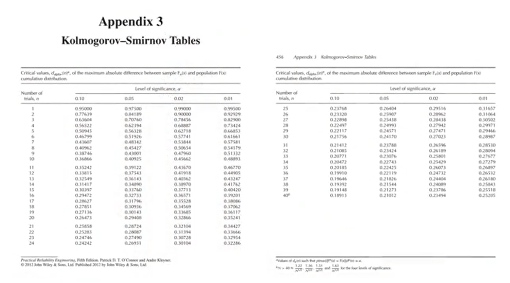
Please note that there are two tables for the Kolmogorov-Smirnov test. One for samples with n less than 40.

So equal sampling units. And one for samples with more than 40 and so, more than 40 sampling units. With also different sampling units, so you need to choose the appropriate one.

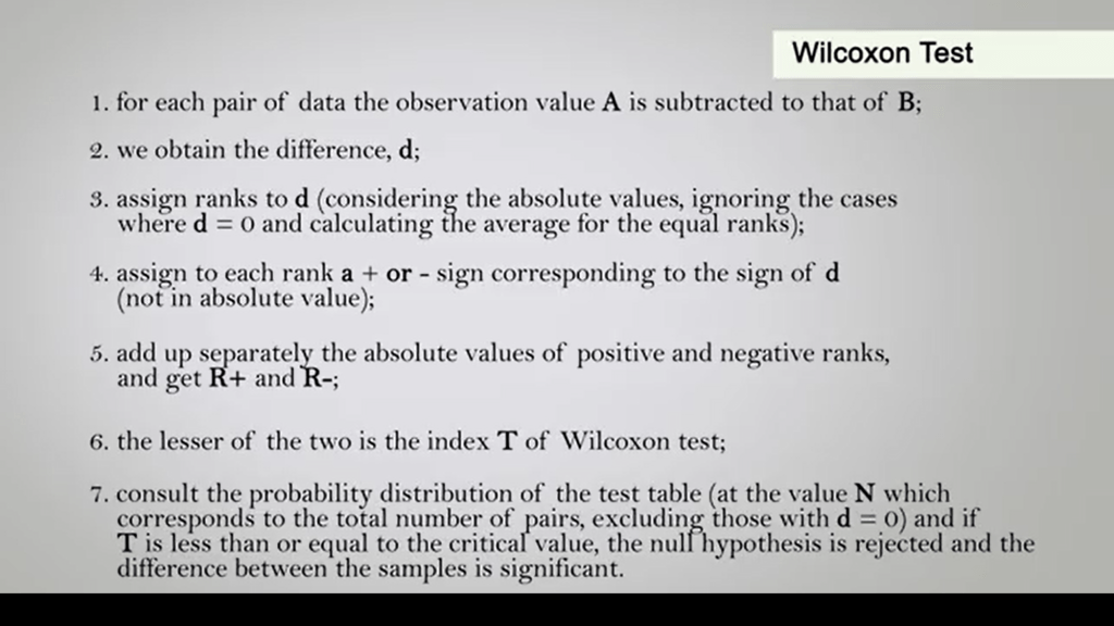
The last non-parametric test I’ll show you today is the Wilcoxon Test. We can use this test when data are paired. In reality, the two samples certainly belong to the same population, but show different characteristics in the observed values. For example, the diameter of the same tree measured what one year of distance or the weight of the same bird, mark it and recapture it after migration. So, to calculate this index, you need to proceed as follow. First, for each pair of data, the observation value A is subtracted to that of B. Then in this case we obtained a difference that is called d. We assigned ranks to d considering the absolute values ignoring the case where d is equal to zero and calculating the average for equal ranks. So, we assign to each rank a plus or minus sign corresponding to the sign of d. Of course, not in absolute value. Then we add up separately the absolute value so positive and negative ranks. And we get our plus and our minus. So, the lesser of the two values is the index T of the Wilcoxon test. So, then we consult the probability distribution of the test table at the value N, which corresponds to the total number of pairs, excluding those with d is equal to 0. And then, if our T value is less than or equal to the critical value, the null hypothesis is rejected, and the difference between the samples is significant. This test can be used only if the total number of pairs excluding those with d is equal to zero, is greater than or equal to six.

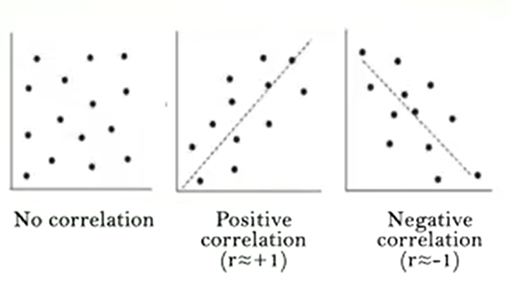
Now we will talk about correlation. We determine correlation we indicate ou rrelationship between two random variables. So that each value of the first variable corresponds with a certain regularity to a value of the second. The correlation cannot be conceded a cause-effect relationship, because it simply is a tendency of a factor to vary in function of another. Sometimes the variation of a variable depends on the variation of the other. For example, the relationship betweenthe eye and the diameter of a tree. But in some cases, there may be other relations or intermediate factors between the two variables. In this case we called them spurious correlations. It is therefore necessary to pay attention to the problems arising from drawing conclusion from the correlations. The correlation is a direct or positive when changing the factor, the other also varies in the same direction.

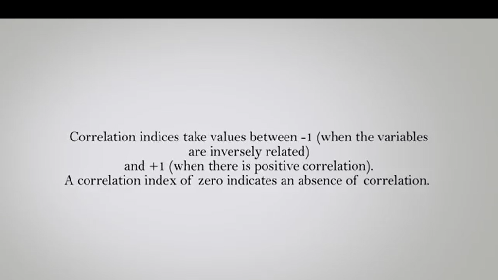
 Why it is an indirect or negative when changing a factor, the other varies in the opposite direction. The degree of correlation between the two variables is expressed by means of correlation indices. These take values between -1,when the variables are inversely related. And +1,when there is a positive correlation. That is when the change of a variable corresponds to a rigidly dependent variation of the other. A correlation index of zero indicates an absence of correlation. Two independent variables havea correlation index equal to zero. But this doesn’t not necessarily imply that the two variables are independent.

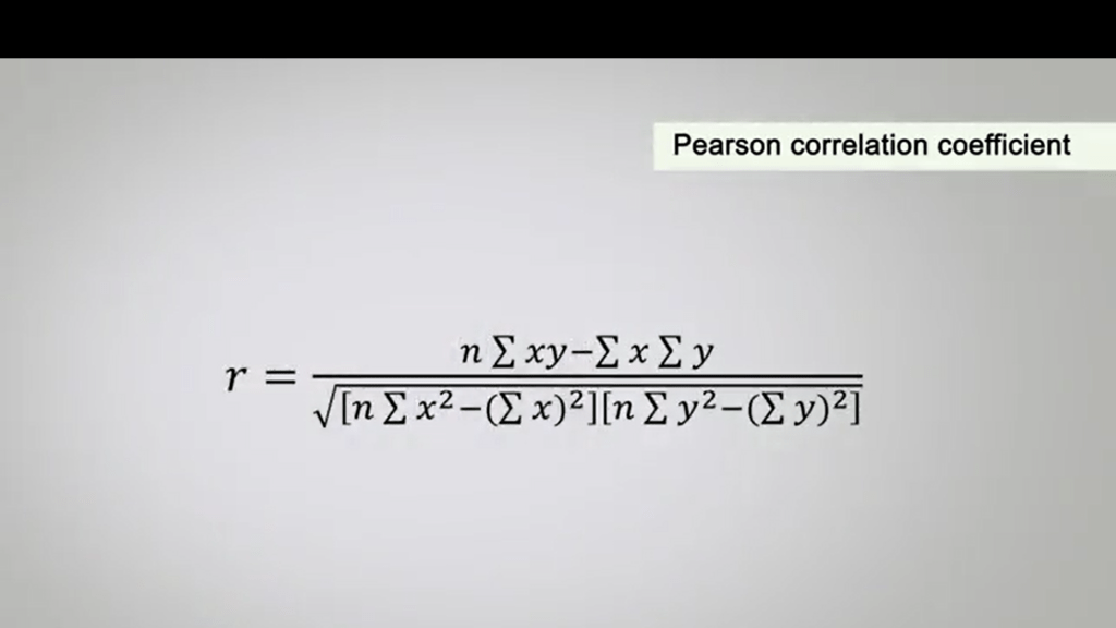
To calculate the correlation coefficient called r Between two factors or variables. For example, i in diameters, length of beak and weight. We need to calculate their means, the square root of errors and the product of the two variables. But in this case, we can calculate the Pearson correlation coefficient. You will see the formula for calculation in this picture.

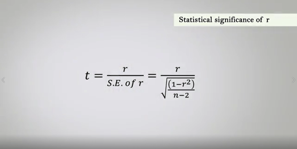
The statistical significance of r can be calculated in the parametric test directly from the tables of the probability of the distribution. Simply dividing r for S.E. So that’s the Standard Error of r. So, you can see that t, in this case, is just r, so the coefficient of correlation divided by the Standard Error of r. The values of t may be compared with those in the table of the critical t statistics. The correspondence of N total minus one, minus one degrees of freedom sowe have N epps and N epsilon.

They are the number of units in the two samples minus two since the variables inthe correlation are two. If the computed values do exceed the critical one to the final level of probability, the correlation is statically significant. The r squared is often called coefficient of determination. And when this is one plus or minus one the correlation positive or negativity is defined it perfect.

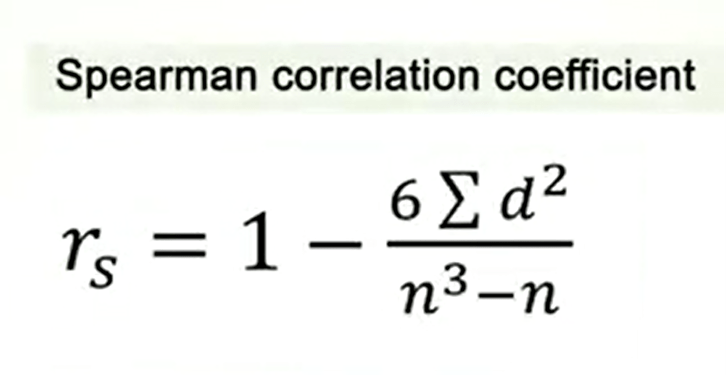
Finally, we must remember then to calculate the correlation and the related coefficient we assume that both sets of data are normally distribution. This is why we calculate the Pearson correlation coefficient. Otherwise, it is necessary to proceed to a normalization using local transformation or the root square. When distribution are be or multi-model, correlation cannot be there. So, a preliminary histogram of the distribution of data we clarify whether the observation are more or less mathematical distributed around one or more values with the largest number of observations. When is that we need to test the significance of a trend. In times serious, when the risk of out of correlation is high and the data are not normally distributed, it is better to use the spearman correlation coefficient. Which employs the ranks of the two variables and the square differences of them, so they are paired. The formula to calculate the spearman correlation coefficient is shown in this picture. So today we saw how correlation works. But we need to understand how to use correlation to calculate for instance regression lines or regression analysis.

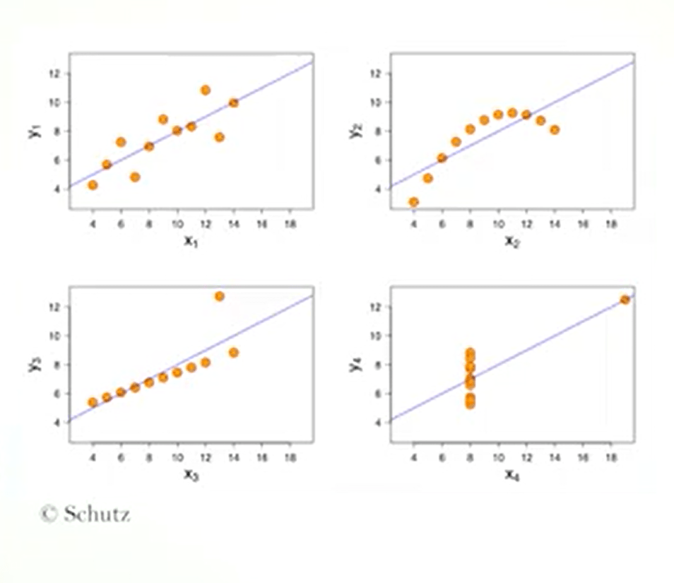
Last time we saw what is a correlation. But we need to understand how to apply correlation to our data. This is the case of regression analysis. If we plot in a graphic two factors or two variables that are assumed to be related to each other, we get a cloud of points. The closer these are, so the correlation coefficient to plus one or minus one, the greater is the distribution along a straight line.

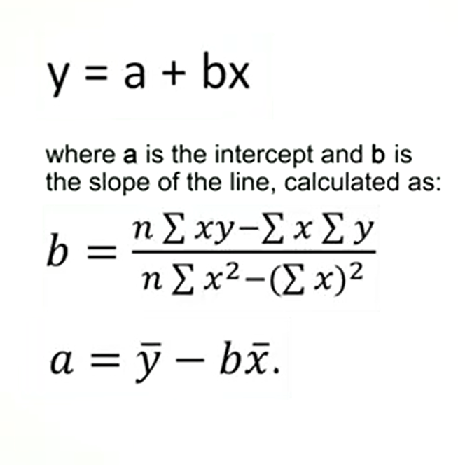
This line is called regression line. And the equation is epsilon equal to a plus b multiplied by x. Where a is the intercept and b is the slope of the line calculated as in this formula. And a is calculated as the mean upsilon minus b mean x.

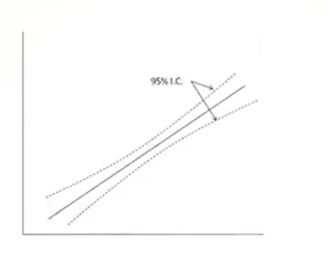
It is possible to identify the confidence lenience of a regression line by creating that zone or interval of confidence above and below the straight line.

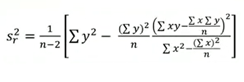
To do this, we must calculate the residual variance, we use this formula to calculate it.

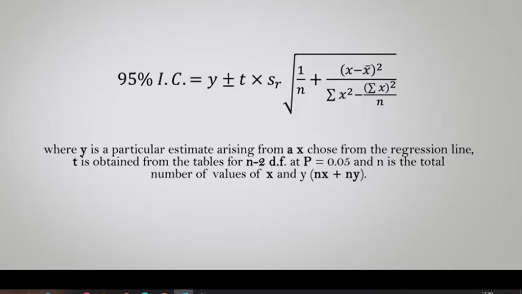
Then, we can estimate the 95% confidence interval. So, 95% of confidence interval, you just calculate by this equation. We use upsilon plus or minus t multiplied by the interval of confidence that we calculate from the residual variance last time. Where in this case, the formula is an upsilon that is a particular estimate arising from x. Choose from this regression line, and t is obtained from the tables forn minus 2 degree of freedom. At P is 0.05 and n sois the total number of values of x and upsilon, so n and x plus n upsilon. Repeating the calculation for many values of upsilon arising from x, it is possible to trace the confidence along the regression line.

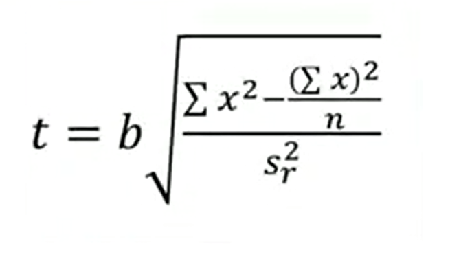
When the points around the regression line are quite dispersed and the coefficient b of the regression line is low, we need to verify the significance of the regression.

Which indicated the probability that there is a real linear relationship between the variable x and the variables upsilon. We use this formula of t. If the calculated value of t, of the related degrees of freedom, in this case n x upsilon minus 2 isgreater than the value in the table, the relationship between the two variables is significant. In ecology, many related variables, may show convenient relationship.

In this case, it is better to transform one of the two variables, usually with the logarithm, or both, until the cartesian graph doesnot show a linear relationship.

Finally, it is important to clarify that the use of our regression analysis, should be limited to cases in which you need to locate the line. That ensure the best approximation of the point in the cloud and while you request an estimate over variable in relation to the other.

When however, we want to measure the degree of our relationship between two variables, the use of the correlation coefficient is more appropriate. If the point are not dispersing symmetrically enough on both sides of the regression line, for all its length, it is recommended to don’t use this type of analysis. An analysis of residuals can be enlightening. When we study, we want to compare the mean of our numbers of samples greater than two we can use a procedure called ANOVA. So, the Analysis of Variants. The Analysis of Variants assumes different names depending on how many the dependent and independent variables are.

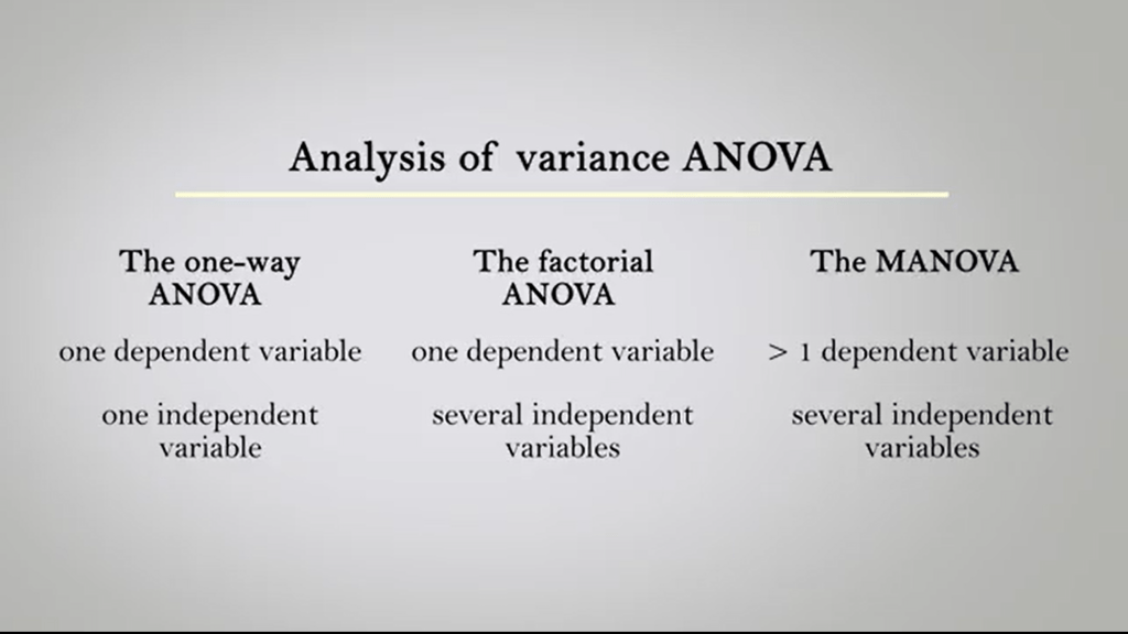
The one-way ANOVA is used is when thereis only one dependent variable, and one independent variable. The factorial ANOVA instead is used for when we have only one dependent variable, and several independent variables. The MANOVA, so the multivariate analysis of variance, is used when we have more than one dependent variables, and several independent variables. The ANOVA technique need can be extended to the analysis of written number factors. The analyzed variable is always one in the ANOVA, but the number of factors or classification criteria or paths that distinguish the different samples is greater than one. This is called a univariate multifactorial ANOVA. There are many statistical software that carry out the calculation of the various type of ANOVA in a few minutes by simply setting the data as required. If we want to compare means of an ecological variable detected in different samples, more than two, the analysis of variance with one criterion or classification, one dependent variable and one independent is the best choice. When instead we want to compare means of a ecological variable detected in different samples, always more than two, but after some time. The best technique is to analyze the variance with two classification criteria. This is an ANOVA which estimates the effect of two independent variables on a dependent variable. Sex and season or weight, for instance. Eye and temperature and diameter, and so soon.