Mathieu GT

Today we will talk about species abundance models.

There are different types of evenness. Type of different patternsare called species abundance models. There are four main types, one isthe geometric series, the second one is the log series, then we have log-normalseries, and broken stick model.

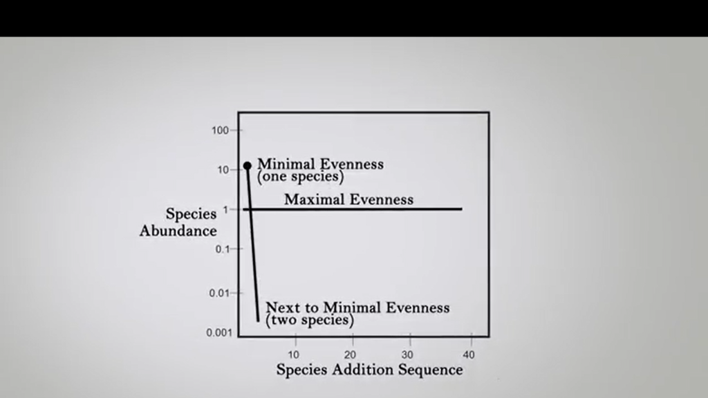
We see that there is a decreasing dominance of a single species from the model one to the model four. So if we try to realize and out these hypothetical to figure out this is a hypothetical molecules are appear, if the maximum evenness will be there, you will see that it’s just a straightline, that is parallel to the x-axis. And when there is minimal evenness, only one species in the sample, for instance, we will see that is the straight line almost close to the parallel line of the epsilon axis.

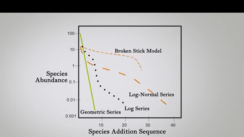
While we want to representdifferent models for evenness distribution by abundance distribution, we can start from the less even, that means that there is only one species or very few species in the samplethat represent the almost parallel line to the epsilon axis, andthis is the geometric series. Then we move more, and we have a kind of log series. The samples is more even, then we have a log-normal series, the evenness is rising. And the last one is the broken stickmodel, that is the maximum even model. So we have difference of the ratio. For instance, evenness increases from geometric series to the log series to the normal series until we reach the broken stickmodels that is the most even sample. So the dominance of having any one species decreases from the geometric to the log to the log-normal to the broken stick models. So broken stick is the closest to the maximum evenness. An important question is, how else could this graph be constructed?

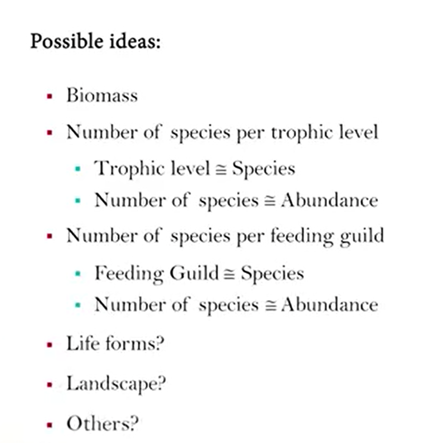
So how will the data there be interpreted? There are possible ideas, for instance, we can build this data on biomass. Or we can build this graph on the number of species per trophic levels where the trophic levels are almost equal to the number of species. And the number of species is almost equal to the abundance, so we can use different variables to build these abundance models. And we can use, for instance, the number of species or feeding guild, where a feeding guild is almost equal to the number of species or life forms or landscapes or other variables.

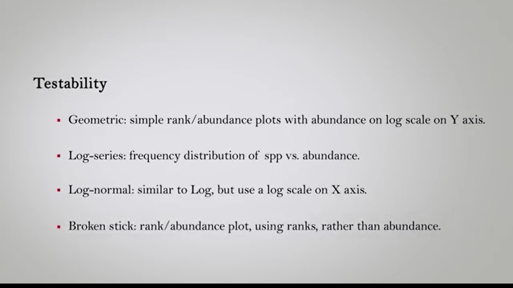
What is very important is the testability because the simple visualization, its inspection of a single group is unsufficient. So how to test each abundance model that differs between each model? In the case of geometric series, we need just simple rank/abundance plots, with abundance on logscale on the epsilon axis. To test the log series stat, we can use the frequency distribution of species versus abundances. For to test the log-normal instead, we use a similar to log, but we can use a log scale on the epsilon axis. To test the broken stick instead, we can use the rank/abundance plot,using ranks, rather than the abundance.

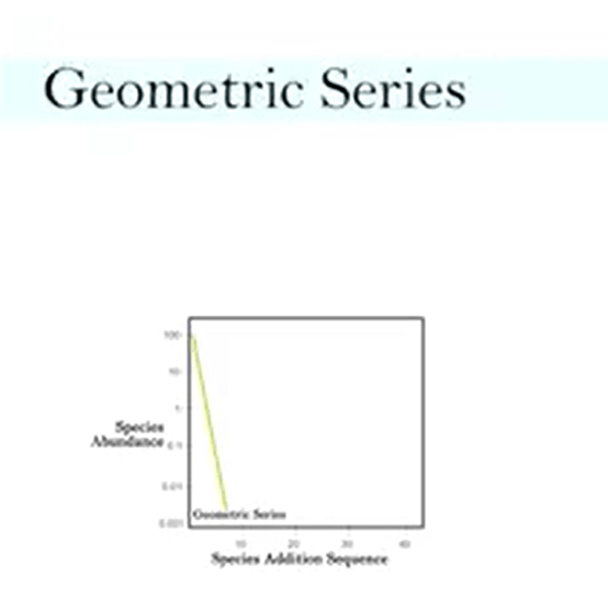
So let’s explain each model in detail. Geometric series, for instance, is a niche preemption, more than the destructionin the ecosystem. So species one, in this case, takesa certain percentage of the resources and prevent other from using them. So it assumes that competitive exclusion or resource exhaustion are the mainforce that influence the series. So then species two takes a bit more. And then it continues with other species until all resources are use it, and those species are included. So you see that geometric series is kind of preemption, a model where minimal cooperation in the ecosystem is assumed.

It also assumes that species abundance is roughly proportional to the total resource use. So we have a linear increase in abundance, that means that there is a linearincrease in the resource use. So interspecific per individual resource use is comparable. So there are not many differences in this,it’s just that the first species takes more than the second that takes more than the third and so on. So mostly common found species poor communities because these model we can see all the worldspecies number is quite low, it means that in this urbansize in polluter size. And this is typical of resuccession, degraded ecosystem, for instance, or richer invaded ecosystem,harsh ecosystems.

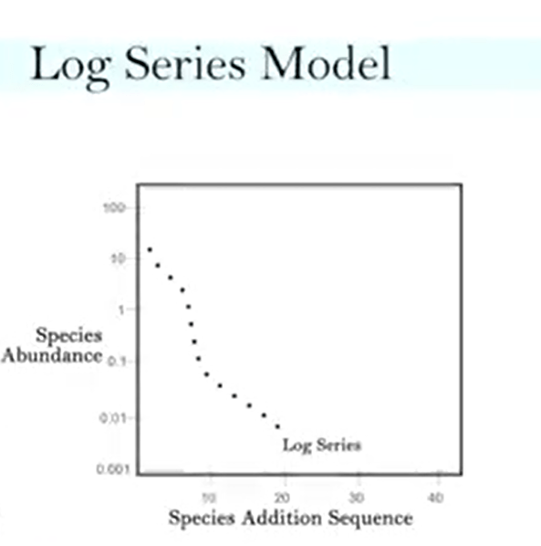
Log series model is that is closely related to geometric series, and some studies have found that both fitting the same data. So this is very similar to geometric and hypothesis about the origin of community, and where the arrival speciesto a normal environment is the same in the geometric series and the log series, but both says that a new factor predominantly structure the community. So both says that one, the geometric ora few in the case of log series species, dominate the total number of species, so dominate a sample. The log series differs from geometric in the assumption about the arrival. For instance, arrival in the log series are randomly arranged. So some species can get some clumpage, some long intervals between arrivals. And in geometric series instead, arrivals are regular and continual.

There is a way to measure the diversity in a log series distribution for its size, and it’s called Alpha-Fisher index. This Fisher index is easy to calculate. It uses an iterate process where you calculate the equation that is from one side just the species total number divided by total abundance, and on the other side, the iterate logarithm of this value. To test the Alpha-Fisher Index is possible to use a statistical test that is called the Kolmogorov’s-Smirnov test, that is one of the best. In this case, we can test if there are differences between two samples on the observer data, and those we expected. This test it’s called goodness of the feed test because it’s already very useful to understand if the distribution of ourdata fit with the log series distribution.

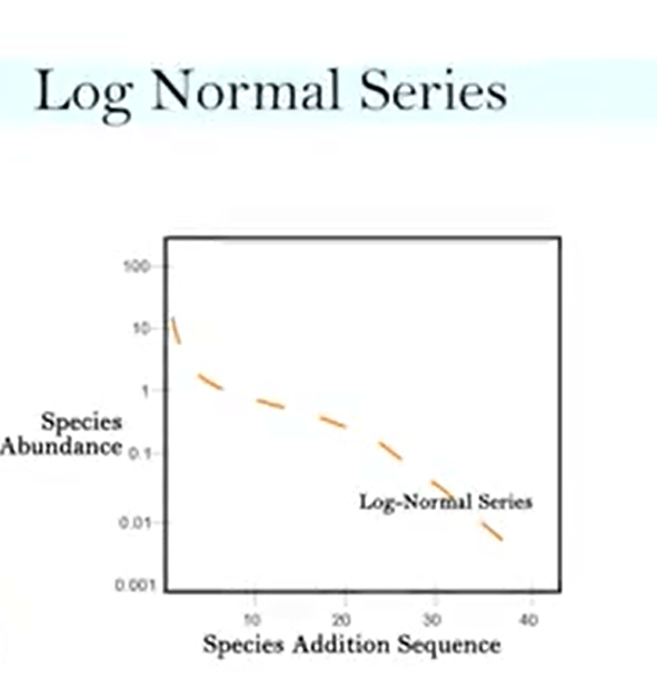
The log-normal series is the most commonin the natural communities, because many data from samples that we can collectin nature fit with the log-normal series. These usually are large measured communities, that’s a representative of large match communities. And for instance, in the temperate forest trees, we usually see this kind ofdistribution on the abundances. Ubiquity, in this case, may be by chance or simple mathematics, so there is a normal distribution that is solved on the consequence of large numbers. This depends also on the central limit theorem, that is the large number factors influence the random variation that will result in normal distribution. So a central assumption is that behind the parameters statistics that the higher is the probability with the higher number factors and more the hour data will fita log-normal distribution. It is a kind of bell shape distribution as explained by Preston with the veil line. That’s why we don’t get rare species, we have the left-side of the distribution that is completely veiled.

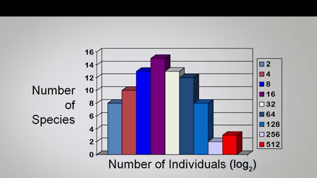
If we look at the picture ofthe histogram representation and we see that species are groupedin two classes according to log2, so they are called octaves. That most common way to represent this data, and any log base can be used any way. In this case if you use octave, so you use log2, we can see that in big samples when we have enough data, we will see this solution in a bell shaped form.

In the log-normal community assembly, there is assumption about a community formation that is the sequential breaking or empty niche space. So each species that arrivessplits the niche space and occupies a niche space that is proportional to its relative abundance. So the probability of niche space being subdivided is independent of its size. In this case, we have a breakage that occur successively. Mechanism that shape the log-normal community can be true in ecological or evolutionary process. And fit to model is not necessary to support the assumption. So we don’t need to test this model to necessarily support the assumption we provide. There are other explanations of this distribution. As I told you, the central limiter theorem, that is not necessary a biological explanation. And another idea, another hypothesis on this distribution, is that species can be divided in three abundance classes. From rare, that are almost 60%,65% of the total number of species, intermediate are almost 25%, andcommon that almost 10% of species. So this shapes are a distribution that we see in our graph. And community saw in this way our composite by batches, batches of group array, intermediate and common species, and the abundance of species that is equal to the sum of the abundance in all batches. So this is an after result ina log-normal distribution.

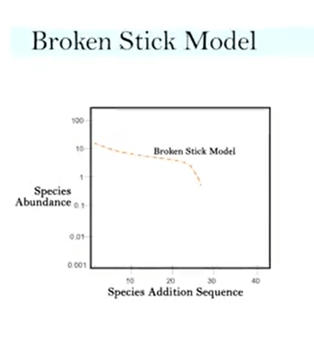
The last model is the broken stick model. Sometimes it’s called random niche boundary hypothesis. Because the broken stick means that you have a stick that is broken in small pieces, so and randomly and simultaneous, it’s broken without any real relationship between early speicies presence and niche size of subsequential arrival. So it is unlike all earlier models, so it’s completely different from them and successfully fit in past. For instance, MacArthur’s show in 1960 that follow this kind of abundance stick, broken stick model, that minnows and King showed in1964 that also follows this. But in general,this model best fit in a narrowly defined communities of taxonomically related organism. So there is no other adequate diversity index needed if data fit broken stick, because if our data fits this broken stickmodel, we don’t have diversity in this. We can use to understand the model or to just explain this model, and we can just use richness, just simple richness, that is another way to measure of thisdiversity in this kind of distribution. Broken stick model also suggests that there is a most equitable species abundance as it will happen naturally, and most biologically realisticuniform distribution. Theoretically, if only we look at one resource, for instance, a space we can explain this broken stick model. But strongly, if this model issubject to sample size when we don’t have crowding limitation between species. So in general, there are limitation to do the model that is not really applicable to a single sample, usually conceived as the average number of species abundance distribution. It can also be misleading to testfate of a single sample to theory of equal resource partitioning. And anyway, the broken stick model is fine to use since we will use it to the other answer to species abundance model. So that’s all for today. Thanks for your attention. I see you next time.