Mathieu GT

Hi, guys. Welcome to the fifth lecture of my course Biological Diversity, Theories, Measure, and Data Sampling Techniques. Today we will talk about beta-diversity. Beta-diversity is just diversity among samples.

There are some relation who link beta, alpha, and gamma-diversity. For instance, gamma-diversity can bea sum of alpha and beta-diversity, or it can be intended as a multiplication between alpha and beta-diversity. So in some cases, if you just from gamma-diversity subtract alpha-diversity, you get beta-diversity. Beta-diversity can be measured in space and in time. Sometimes we can measure beta-diversity as a difference in alpha-diversity. And most of these indexes use presence/absence data that are, of course, incidence data.

For instance, one of them is the beta-diversity of Whittaker. That’s simply the number of species, S, the total number of species of the area. That means, for instance, gamma-diversity. Divided by alpha, that is, the mean diversity of the samples. But there are some conditionto calculate this index. For instance, we need that samples have the same dimension, that diversity is measured as a species richness, and then one is the maximum similarity that we can get from this index and two is the minimum similarity.

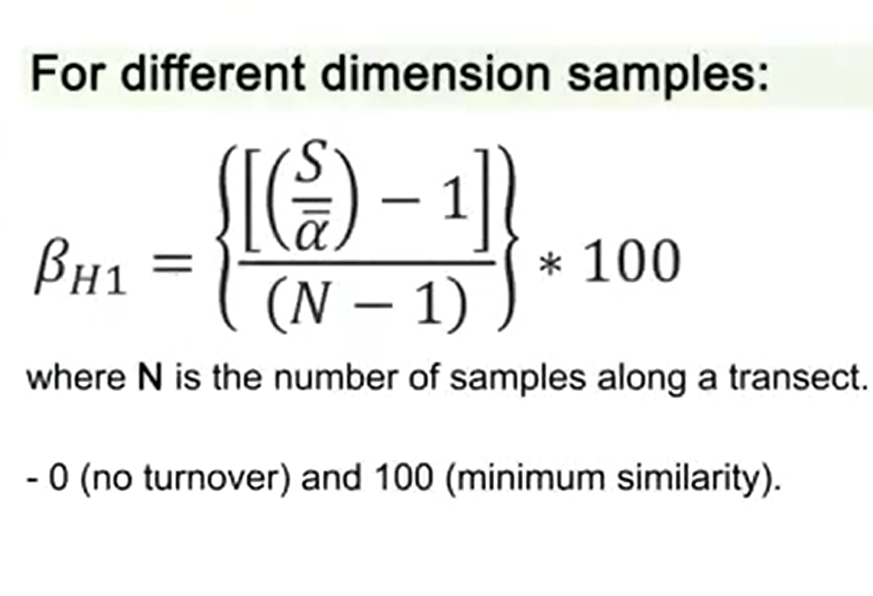
If we have samples of different dimension, we can calculate another index that is just the same Whittaker that is subtracted by 1 divided by N-1 multiplied by 100. That is N, just the number of samples along the transect. So if we have a transect, we measure the number of samples and then we divide this number by the Whittaker index. In this case, we have 0 as in no turnover, that is no diversity, and 100 that is minimum similarity.

That is that the samples have very low similarity means that beta-diversity is high.

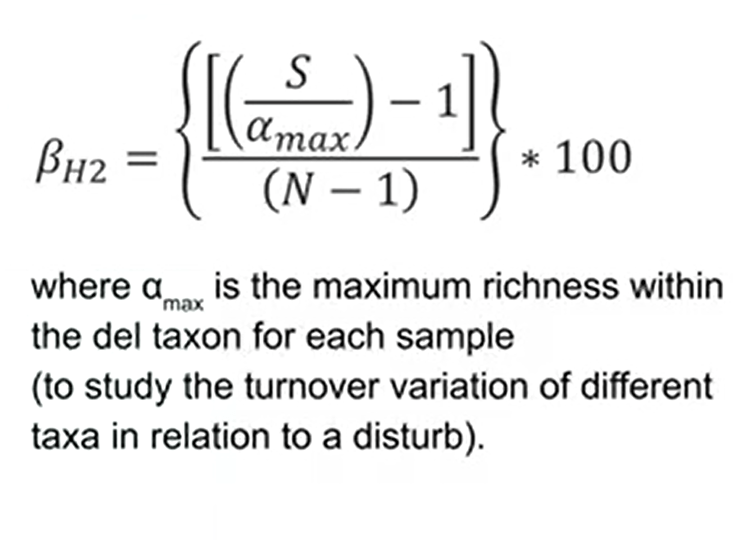
If we want to understand when species are lost and others are gained, there’s an index that is not influenced by trends of species richness and is the same of previous one, but is not divided by alpha min but is divided by alpha max. That is the maximum richness within the taxon, for example, so this is useful to study the turnover variation of different taxa in relation to a disturb.

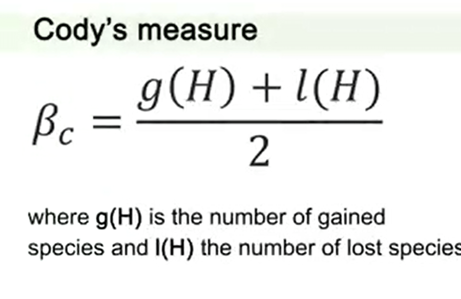
Another measure is the Cody measure or Cody index that sums the number of species gained along a transect to the number of species lost. So we have the number g, that is number of species gained, plus l that’s the number of species lost, divided by 2. This is also another index to measure differences in alpha-diversity.

Then there are three indexes that are called Routledge indexes that are based on the decomposition of alpha and beta-diversity. One of them is just the square value of total species richness divided by (2r+S)-1,where r is just the number of couples of species with overlapping distributions.

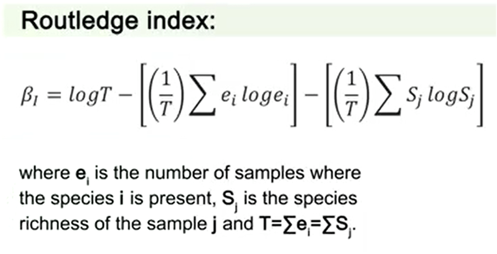
The second of the three Routledge indexes is for incidence data and needs samples of the same dimension. You will see the formula in the picture, where e is just the number of samples where the species i is present, S j is the species richness of the sample j.

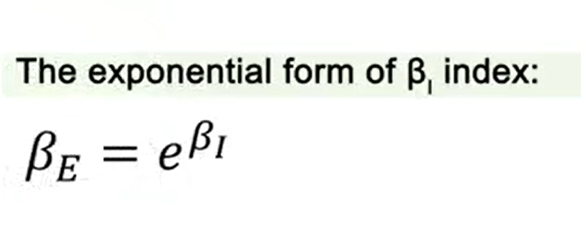
There is another version, that is the exponential form of the Routledge index, and it’s just the exponential of B I, so this is the second index that I show you in the exponential form.

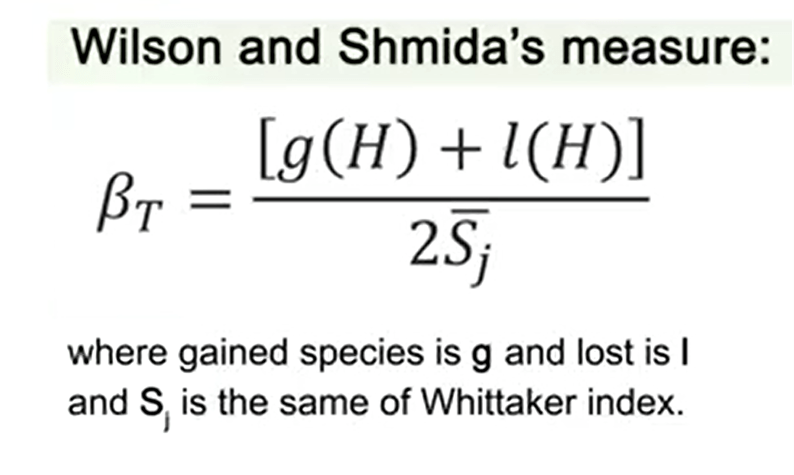
The last measure of differences in alpha-diversity that I present you is the Wilson and Shmida’s. This index is just the sum of gained species plus the number of lost species divided by 2 multiplied by S j that is the same of Whittaker index. In general, Whittaker, I mean beta W, index is just the best performing measure.

If we want to measure beta-diversity in space, so we want to understand complementary and similarity, and in this case we want to know if there is a low spatial turnover or high spatial turnover, it’s interesting to understand how this similarity can be calculated.

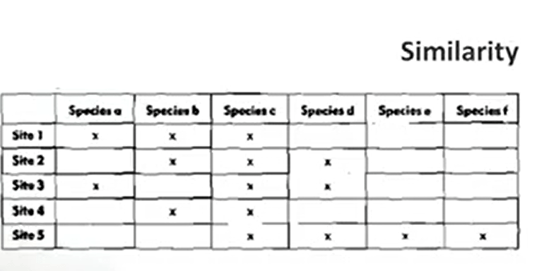
For instance, if we want to measure, to understand which of the samples that we have or which of theare as that we have in a specific space, is the best to reachthe highest number of species. So we have area one, as an example in this table, that the Site 1 has Species a, Species b, Species c, but not d, e, and f, and Site 5 that has Species c, Species d, Species e, and f. In this case, the best combination of these sites is Site 1 and Site 5, and this way we get a highest number of species, if we want to set, for instance, a protected area.

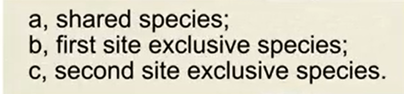
 So all these indexes has the same three variables that are a, b, and c, where a is the number of shared species, b is the first site exclusive species, and c is the second site exclusive species.

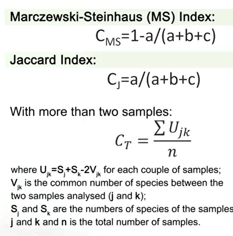
The Marczewski-Steinhaus index is just calculated as 1-a divided by (a +b+c). It is just the complemental form of the famous Jaccard index that is the same instead 1 minus. So just remove 1 minus, you get the Jaccard index. That’s very useful and very easy to calculate. When you have more than two samples, you can just use a different formula that divided the sum of U jk divided by n. Where U jk is just the couple of samples that is summed with the V jk that’s the common numbers species between the two samples analyzed, j and k, and S j and S k is the number of species of sample j and sample k, and n, the total number of samples.

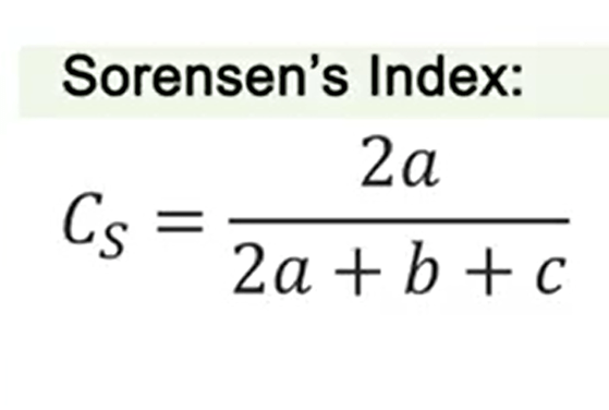
Another very famous indexis Sorensen’s index. This index divide 2 multiplied by a, that as I told you is the variable of shared species,divided by 2 multiplied by a+b+c. It’s one of the most efficient of the measures for complementarity and similarity. But if the differences of S,so the total species number, is i, the results are always i.

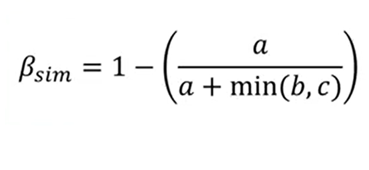
A new version of this index has been provided to reduce this effect. This index is just 1-(adivided by a+min(b,c)).

There are some other indexes that are based on abundances. One of them is the Bray-Curtis index, that modified version of Sorensen index. In this case we have that the index is just 2 multiplied by j multiplied by N divided by (N a + N b), where Na is the total abundance of the site a, N b is the total abundance of the site b,and 2 multiplied j N is the sum of the minimum abundance values of both sites, so it’s the min(n a) and the min(n b).

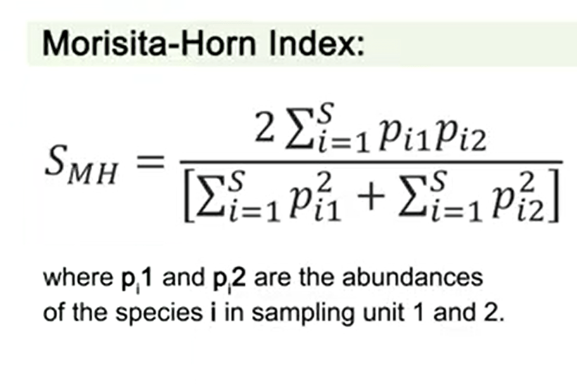
All the previous measures are influenced by the richness and the examples I mentioned, but there is one that is not so affected, and is the Morisita-Horn index, that is not but influenced by the most abundance pieces.

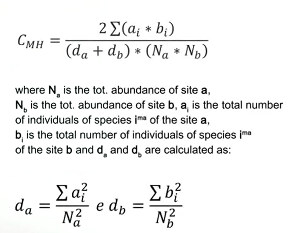
When we want to give less weight to abundant species, we use a modified version of the Morisita-Horn index. That is this one provided in the formula, where N a is the total abundance of site a, N b is the total abundance of the site b, and a i is the total abundance of individuals of species in the site a, b i is the total abundance of the speciesism of the site b, and d a and d b are calculated asthe formulas that are provided here.

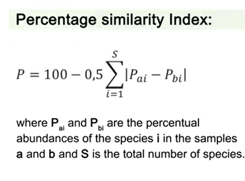
Another interesting index of similarity is the percentage similarity index. In this case we subtract by 100-0.5 and the sum of P ai and P bi, where P ai and P bi are the percentual abundances of the species i in the samples a and b, and S is the total number of species.

So in this plethora of indexes we need to understand which one is the best. And usually Whittaker, or beta W index for differences in alpha-diversity, is one of the best when want to analyze differences in alpha-diversity. Sorensen index and Bray-Curtis index are some of the best for incidence data, so when we have data on presence, absence data. And the Morisita-Hornindex is the best for abundance data when we have the abundances of the species.

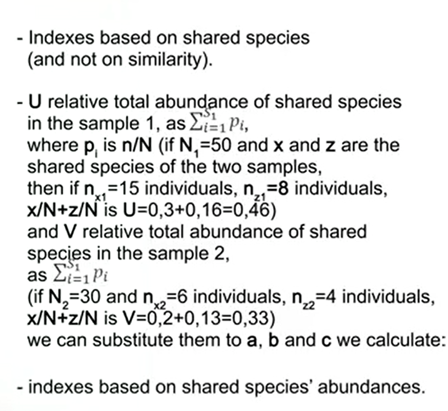
There are also beta-diversity indices inspace that account for shared species, so they are not based on similarity but onthe species that are shared among samples. In these indexes we havedifferent variables. One of these the U, that isthe relative total abundance of shared species in the sample 1, as the sum ofthe p i, that where p i is n divided by N. So if we have total abundance of 50,and x and z are the shared speciesof the two samples, then if n x is 15 individuals andn z is 8 individuals, we have that x divided by N + zdivided by N is U = 0.3+0.16=0.46.

And the other viable is V, that is the relative total abundance or shared species in the sample 2. It is calculated as the previous one, as the sum of p i. So if we have N 2 that is the total 30 individuals as a total abundance and n x that is 6 individuals andn z that is 4 individuals, then we have that x dividedby n + z divided by n is V=0.2+0.13 that is total 0.33.

And then we can substitute them to a,b, and c of the previous formulas that I already show you to calculate indexes based on shared species abundances.

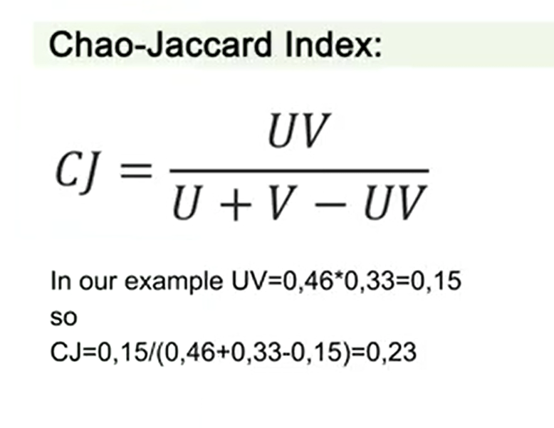
One of these is the Chao-Jaccard index. The Chao-Jaccard index is just Umultiplied by V, divided by U+V-UV. In our example, for instance,U multiplied by V is 0.46 multiplied by 0.32, that’s total of 0.15. So the Chao-Jaccard index inthis case is U multiplied by V, that is 0.15, divided by the sumof these three variables, that is 0.46+0.33-0.15,and total number is 0.23. So the Chao-Jaccard index total is 0.23.

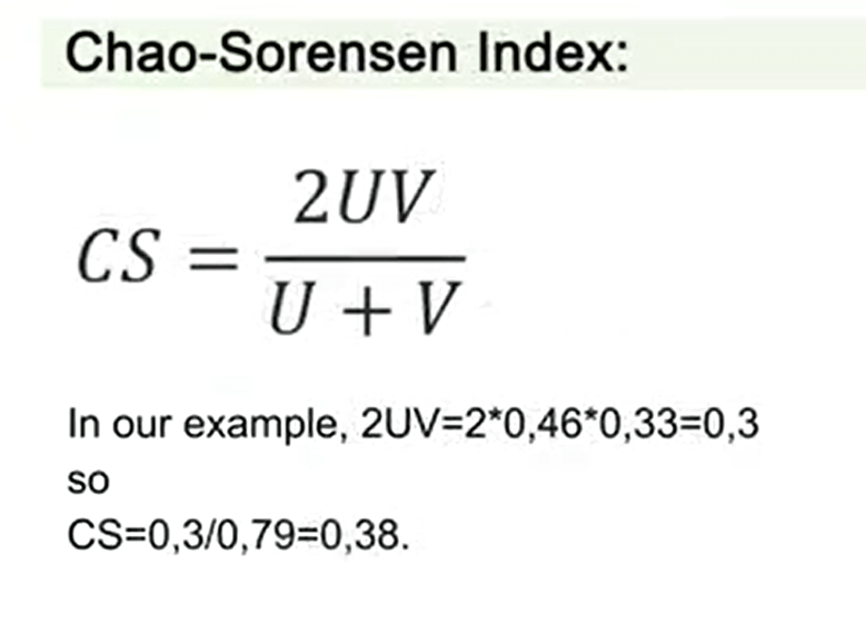
The Chao-Sorensen index is very similarto this one but is 2UV divided by U+V. So in this case, in our example,we have 2UV, that is, 2 multiplied 0.46 multiplied 0.33,and we have a total of 0.3. So the Chao-Sorensen index is just0.3 divided 0.79 to get 0.38.

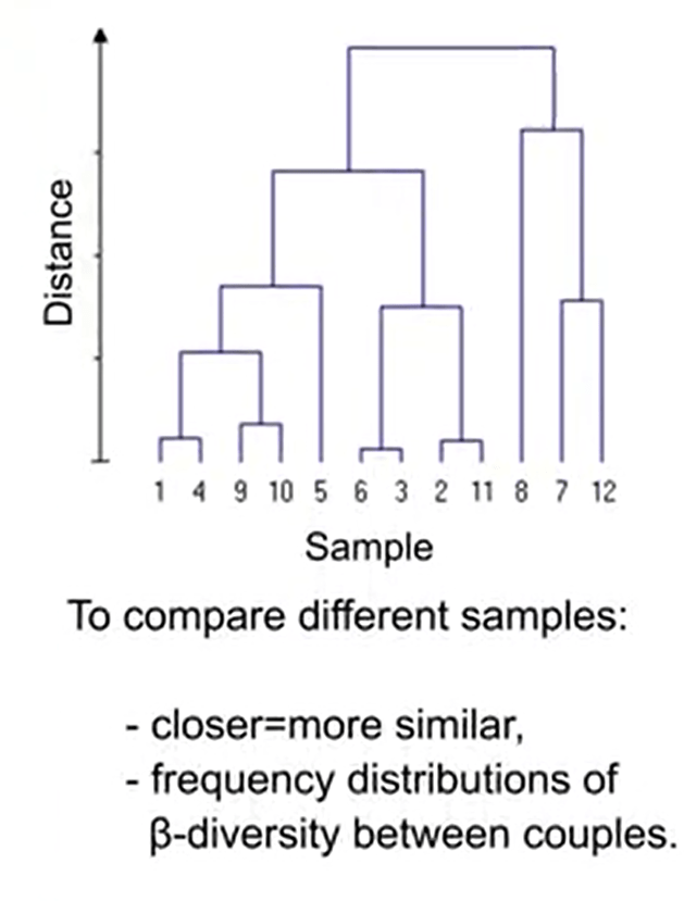
If our samples are from a local scale, it’s better to don’t use complementarity and similarity index, and prefer those based on differences on local diversity. When we want to compare different samples, we have different graphical representation. That can be the cluster analysis wherecloser means that they’re more similar, dendrograms that are frequencydistribution of beta-diversity couples. So we can use these different ways tounderstand the differences between our samples.

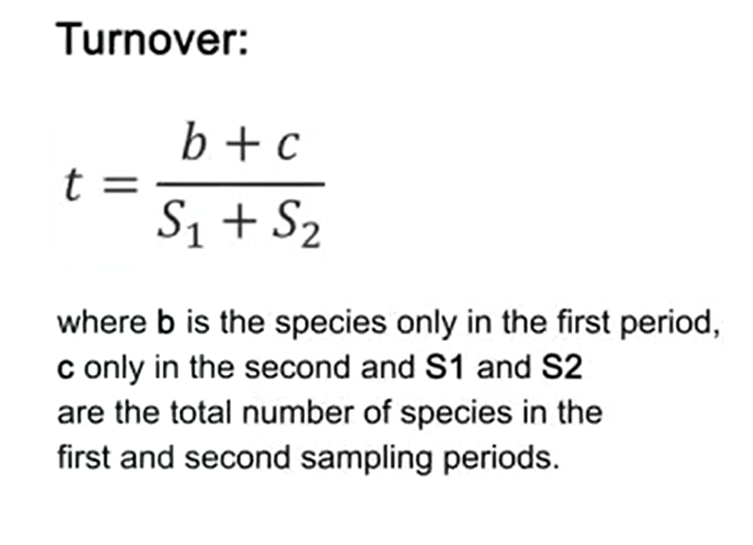
There is also a way to calculate the changes in beta-diversity so differences among the samples, but in time. Imagine you go to a field and measure what’s diversity in that samples and then after ten years, for instance, you go there again in the same place and you want to understand what’s the difference, how beta-diversity changed, how diversity in general changed. This is kind of turnover time orturnover diversity, and to measure this turnover diversity we can use just the simple formula thatis b+c divided S 1 + S 2. Where b is the number of species of only the first period, so the first time we went in the field, c is only the second period, the species that are collectedonly in the second time, S 1 and S 2 are the total number of species in the first and the second sampling period.

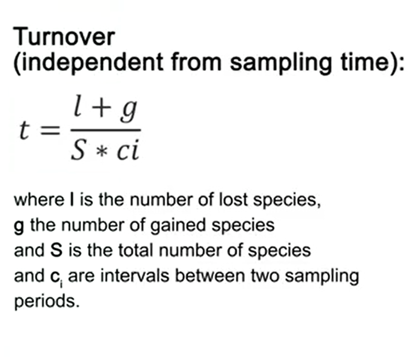
We have another way to calculate the turnover independent from the sampling time. That is simply l+g divided by S multiplied by ci, where l is the number of lost species, g is the number of gained species, and S is the total number of species where ci is the interval between two sampling. Thank you for your attention. I will provide some tables with data to calculate this index I already show you. See you next time.